

On this page
The indefinite integral ∫ √(tan x) dx is legendary among high school and engineering entrance students because direct integration methods fail immediately. Standard substitutions like t = tan x yield 1 / (2 √t (1 + t²)), which resists straightforward partial fractions without first rationalising the radical. In the official Class 12 curriculum published by the Central Board of Secondary Education (CBSE Academic Curriculum), calculus carries 35 out of 80 total theory marks, making advanced integration techniques essential. The National Testing Agency also tests structural transformations in competitive exams like JEE Main, where recognizing hidden symmetry saves valuable minutes during problem solving.
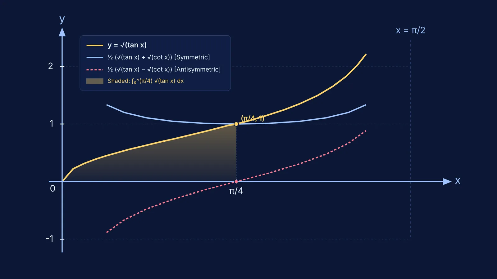
The secret to conquering ∫ √(tan x) dx lies in decomposing √(tan x) into the arithmetic mean of two complementary parts: a symmetric sum and an antisymmetric difference involving its reciprocal, √(cot x). Transforming non-rational integrands through structured algebraic substitutions is a foundational technique in analysis (Wolfram MathWorld). By converting each half into a standard rational expression, you can apply paired quadratic substitutions that integrate cleanly into elementary functions.
How do you split root tan x into symmetric halves?
Because cot x is the reciprocal of tan x, we have √(cot x) = 1 / √(tan x). We can write √(tan x) identically as:
√(tan x) = (1/2) [ (√(tan x) + √(cot x)) + (√(tan x) − √(cot x)) ]
This identity splits I = ∫ √(tan x) dx into two separate integrals:
I = (1/2) I₁ + (1/2) I₂
where I₁ = ∫ (√(tan x) + √(cot x)) dx and I₂ = ∫ (√(tan x) − √(cot x)) dx.
To express both integrals algebraically, substitute t = √(tan x). Then t² = tan x, and differentiating gives 2t dt = sec² x dx = (1 + t⁴) dx, which means dx = 2t dt / (1 + t⁴).
Substituting into each integral gives:
For I₁: √(tan x) + √(cot x) = (t² + 1) / t, so:
I₁ = ∫ [ (t² + 1) / t ] · [ 2t dt / (1 + t⁴) ] = 2 ∫ (t² + 1) / (t⁴ + 1) dt
For I₂: √(tan x) − √(cot x) = (t² − 1) / t, so:
I₂ = ∫ [ (t² − 1) / t ] · [ 2t dt / (1 + t⁴) ] = 2 ∫ (t² − 1) / (t⁴ + 1) dt
Dividing numerator and denominator by t² produces standard forms:
I₁ = 2 ∫ (1 + 1/t²) / (t² + 1/t²) dt
I₂ = 2 ∫ (1 − 1/t²) / (t² + 1/t²) dt
Students looking for guidance on substitution strategies often refer to choosing the right substitution variable. The Fermi Problem Library has worked problems with a step-by-step solver that explains the reasoning rather than printing an answer, helping you verify each stage of the algebraic transformation.
How do the substitutions u and v resolve the two integrals?
In I₁ and I₂, the numerators match the exact derivatives of reciprocal combinations: (1 + 1/t²) dt is d(t − 1/t), while (1 − 1/t²) dt is d(t + 1/t). This motivates two paired substitutions:
For the first integral I₁:
Let u = t − 1/t = (tan x − 1) / √(tan x).
Then du = (1 + 1/t²) dt, and u² = t² + 1/t² − 2, giving t² + 1/t² = u² + 2.
Substituting into I₁ gives: I₁ = 2 ∫ du / (u² + 2) = 2 · (1/√2) arctan(u / √2) = √2 arctan( (tan x − 1) / √(2 tan x) )
For the second integral I₂:
Let v = t + 1/t = (tan x + 1) / √(tan x).
Then dv = (1 − 1/t²) dt, and v² = t² + 1/t² + 2, giving t² + 1/t² = v² − 2.
Using the standard logarithmic formula for integrals with quadratic denominators: I₂ = 2 ∫ dv / (v² − 2) = 2 · [ 1 / (2√2) ] ln | (v − √2) / (v + √2) | = (1/√2) ln | (v − √2) / (v + √2) |
Substituting back v yields: I₂ = (1/√2) ln | (tan x − √(2 tan x) + 1) / (tan x + √(2 tan x) + 1) |
What is the final assembled integral of root tan x?
Reassembling both halves into I = (1/2) I₁ + (1/2) I₂ and adding the constant of integration C produces the complete antiderivative:
∫ √(tan x) dx = (1/√2) arctan( (tan x − 1) / √(2 tan x) ) + (1 / (2√2)) ln | (tan x − √(2 tan x) + 1) / (tan x + √(2 tan x) + 1) | + C
Evaluating at x = π/4 confirms continuity across the first quadrant:
At x = π/4, tan(π/4) = 1, so the arctan argument becomes 0, yielding arctan(0) = 0.
The logarithmic argument reduces to (2 − √2) / (2 + √2) = (√2 − 1)².
Both terms yield finite real values, verifying that the antiderivative remains smooth.
When preparing for exams with multi-step calculus problems, following a structured four-week integration practice plan ensures you master these algebraic patterns across mixed problem sets. If you get stuck identifying intermediate steps, Fermi's AI tutor notices where a student is stuck and decides whether to explain, ask, or show the next step.
Why do textbook answers use arctan while some use arcsin?
Students comparing solutions across reference textbooks often encounter an alternative expression for I₁: I₁ = √2 arcsin(sin x − cos x)
This form arises by converting the integrand into sines and cosines before substituting: √(tan x) + √(cot x) = (sin x + cos x) / √(sin x cos x) = √2 (sin x + cos x) / √(sin 2x)
Letting w = sin x − cos x gives dw = (cos x + sin x) dx and sin 2x = 1 − w², transforming I₁ into √2 ∫ dw / √(1 − w²) = √2 arcsin(sin x − cos x).
The two forms are identical on the domain where tan x > 0. In a right triangle with opposite side (tan x − 1) and adjacent side √(2 tan x), the hypotenuse is √(tan² x + 1) = sec x. The sine of this angle is (tan x − 1) / sec x = sin x − cos x, proving that arctan( (tan x − 1) / √(2 tan x) ) = arcsin(sin x − cos x).
The algebraic arctan form remains standard because it mirrors the rational denominator decomposition. Mapping both representations within the Fermi Concept Library connects trigonometric substitution with polynomial factoring, clarifying how distinct calculus techniques arrive at the same analytical truth.


