

On this page
Integrating a modulus function directly often leads to sign errors. The safest approach is to remove the absolute value bars by splitting the definite integral into intervals where the inside expression is clearly positive or negative. We can then verify the algebraic result using basic geometry, building a deeper intuition for how these functions behave.
Where do you split the modulus integral?
The expression inside the modulus is x − 1. This expression changes sign when x − 1 = 0, which happens at the critical point x = 1.
This critical point lies exactly in the middle of our integration limits (from x = 0 to x = 2). We use the property of definite integrals that allows us to break the path of integration at any point c between a and b:
∫ (from 0 to 2) |x − 1| dx = ∫ (from 0 to 1) |x − 1| dx + ∫ (from 1 to 2) |x − 1| dx
Now we examine the sign of x − 1 in each interval to remove the modulus bars safely:
For x between 0 and 1, the expression x − 1 is negative. Therefore, we must flip its sign to make it positive: |x − 1| = −(x − 1) = 1 − x.
For x between 1 and 2, the expression x − 1 is already positive. Therefore, the absolute value leaves it unchanged: |x − 1| = x − 1.
Substituting these piecewise expressions back gives standard polynomial integrals:
∫ (from 0 to 1) (1 − x) dx + ∫ (from 1 to 2) (x − 1) dx
Evaluating the first part: [x − x²/2] from 0 to 1 = (1 − 1/2) − (0) = 1/2.
Evaluating the second part: [x²/2 − x] from 1 to 2 = (4/2 − 2) − (1/2 − 1) = (2 − 2) − (−1/2) = 1/2.
Adding them together, the total integral is 1/2 + 1/2 = 1.
How do you check your answer with geometry?
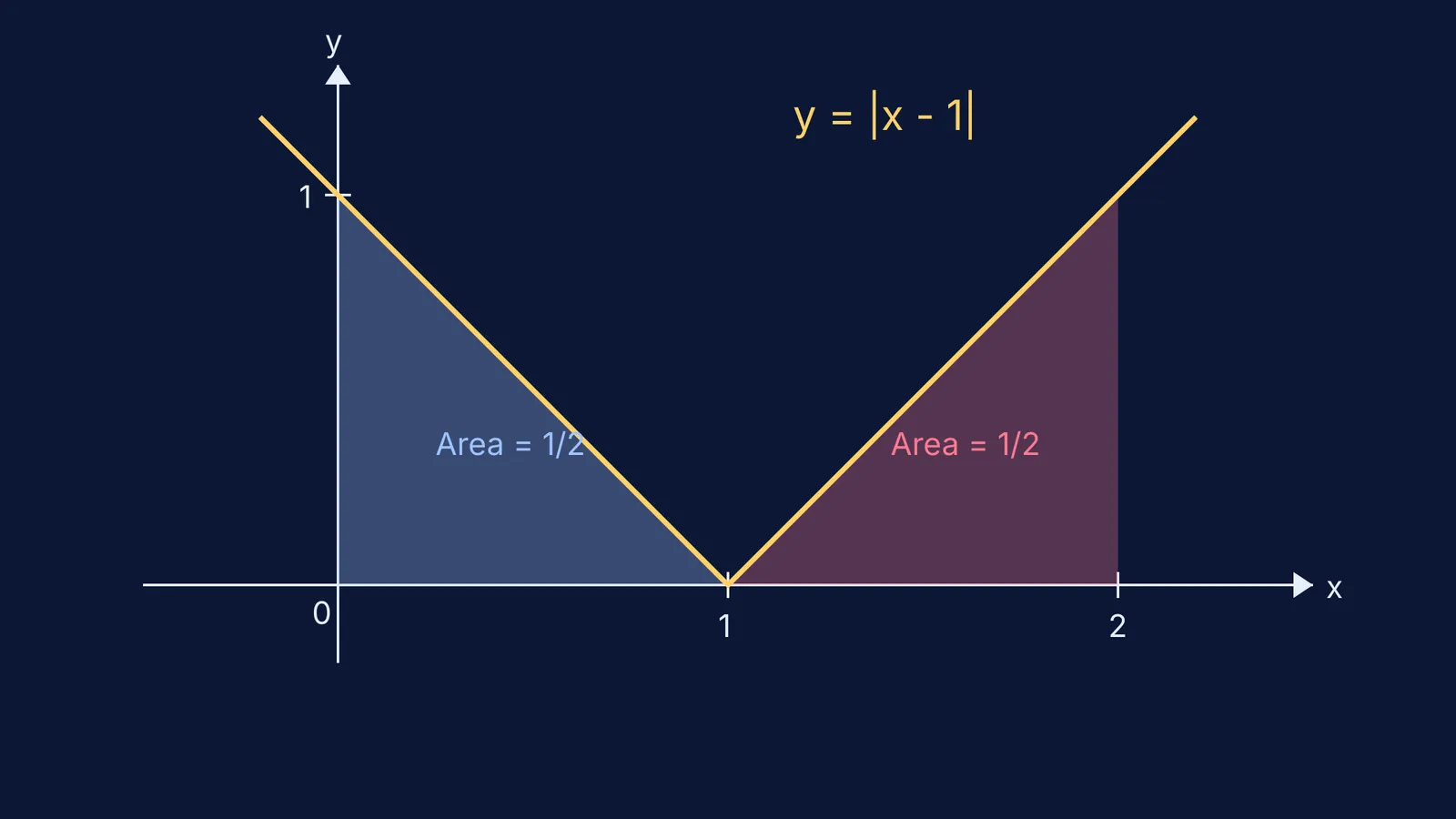
Definite integrals represent the area under a curve. The graph of y = |x − 1| is a V-shaped set of intersecting lines with its lowest point, the vertex, resting at (1, 0). When you plot this function between x = 0 and x = 2, the region bounded by the curve and the x-axis forms two right-angled triangles.
The left triangle runs from x = 0 to x = 1. Its base is 1 unit long, and its height at x = 0 is |0 − 1| = 1. Its area is 1/2 × base × height = 1/2.
The right triangle runs from x = 1 to x = 2. Its base is 1 unit long, and its height at x = 2 is |2 − 1| = 1. Its area is also 1/2 × 1 × 1 = 1/2.
Summing these geometric areas gives 1/2 + 1/2 = 1. This geometric method serves as a fast and reliable check against your algebraic integration, ensuring no negative signs were dropped along the way.
Why does the modulus function need splitting?
One 2012 study of high school students published in *Educational Studies in Mathematics* found that many learners rely on procedural rules to solve absolute value problems rather than understanding the underlying distance definition. You cannot apply the standard power rule of integration directly to an expression like |x − 1| because the modulus is not a single, continuous polynomial; it is a piecewise function joined at the vertex.
By splitting the domain at the exact point where the inner expression equals zero, you turn the piecewise function back into distinct, ordinary polynomials that follow standard integration rules. This technique is universal, whether you are solving basic modulus equations and inequalities or dealing with complex definite integrals with modulus and floor functions in competitive exams.
What are common mistakes with modulus integrals?
The most frequent error students make is integrating the expression as if the modulus bars were simple parentheses. This incorrect step yields [x²/2 − x] evaluated from 0 to 2, which results in exactly zero. The modulus bars exist specifically to ensure the accumulated area remains entirely positive, which is why the actual result is 1.
In a physics context, if y = |x − 1| represents the speed of an object (which must be positive) while its velocity changes direction at x = 1, the integral from 0 to 2 represents the total distance travelled. If you mistakenly drop the absolute value bars, you would calculate the net displacement, which is zero, instead of the true distance.
If you are unsure where to split a function or how to apply the properties of definite integrals, the Fermi Problem Library has worked problems with a step-by-step solver that explains the reasoning rather than printing an answer. This helps build the habit of visualising the graph before jumping straight into the algebra.


