

On this page
When an electric current passes through a circular loop of radius R, it sets up a magnetic field around every segment of wire. Applying the Biot-Savart law along the central perpendicular axis gives the familiar axial field formula: B(x) = μ₀ N I R² / [2 (R² + x²)³/²], where N is the number of turns and I is the current. At the exact centre of the loop (x = 0), the magnetic field reaches its maximum value, B_c = μ₀ N I / (2R).
Why does a single circular coil fail to provide a uniform magnetic field?
The limitation of a single loop becomes obvious as soon as you step away from its centre. Because axial distance x enters the denominator as (R² + x²)³/², the field falls off steeply. As shown in Revista Brasileira de Ensino de Física, at half a radius away (x = R/2), the field drops to roughly 71.6% of its peak value; at a full radius (x = R), it drops to barely 35.4%. For experiments like steering electron beams or calibrating sensors, this steep drop across a few centimetres is far too uneven.
In 1849, Hermann von Helmholtz solved this while improving Claude Pouillet's 1837 tangent galvanometer, as noted in Nature. In Pouillet's instrument, compass needle tips swung into weaker fields during large deflections, causing non-linear errors. Helmholtz realized that pairing two identical coils could eliminate this field decay.
How does adding two coaxial coils cancel the field curvature?
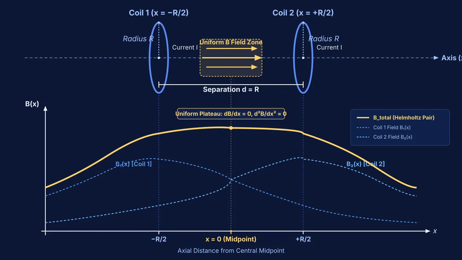
Consider two identical circular coils of radius R with N turns, carrying current I in the same direction at coaxial separation d. Setting origin x = 0 at their midpoint places Coil 1 at x = −d/2 and Coil 2 at x = +d/2. By linear superposition, the total axial field is:
B_total(x) = (μ₀ N I R² / 2) × [ (R² + (x + d/2)²)⁻³/² + (R² + (x − d/2)²)⁻³/² ]
Reflective symmetry ensures that moving away from x = 0 increases distance to one coil by the same amount it decreases distance to the other. Their slopes cancel identically, giving dB_total/dx = 0 at x = 0 for any separation d.
However, zero slope only creates a stationary point. If coils are too far apart, the field dips at the centre; if too close, it peaks. Differentiating a single coil's axial field twice with respect to x gives:
d²B/dx² = [3 μ₀ N I R² / 2] × (4x² − R²) / (R² + x²)⁷/²
This curvature vanishes at 4x² − R² = 0, or x = ± R/2. Each coil possesses natural inflection points at half its radius. Setting coil separation equal to radius (d = R) places the midpoint at R/2 from both coils. As shown in Revista Brasileira de Ensino de Física, the concave-up profile of one coil cancels the concave-down profile of the other. In the American Journal of Physics, Edward M. Purcell demonstrated that d = R also cancels the magnetic octupole moment, leaving the fourth derivative as the first non-vanishing term.
What is the magnetic field formula at the midpoint between the coils?
Substituting x = 0 and d = R into the superposition equation gives the central field, as formulated in Revista Brasileira de Ensino de Física:
At x = 0, each coil lies at axial distance R/2, giving R² + (R/2)² = 5R²/4.
Raising this term to the power of 3/2 gives (5/4)³/² R³ = (5√5 / 8) R³.
The field contributed by a single coil is B₁(0) = (μ₀ N I R²) / [2 × (5√5 / 8) R³] = (4 / 5√5) × (μ₀ N I / R).
Adding both coils gives B_total(0) = (8 / 5√5) × (μ₀ N I / R) = (4/5)³/² × (μ₀ N I / R) ≈ 0.7155 × (μ₀ N I / R).
Comparing this to the central field of a single isolated coil, B_c = μ₀ N I / (2R), the Helmholtz midpoint field is B_total(0) = (16 / 5√5) B_c ≈ 1.431 B_c.
Consider a standard laboratory setup: two coaxial coils of radius R = 0.10 m, each with N = 100 turns, carry a current of I = 2.0 A in series. Using μ₀ = 4π × 10⁻⁷ T·m/A:
B_total(0) = (8 / (5√5)) × [ (4π × 10⁻⁷ T·m/A × 100 × 2.0 A) / 0.10 m ] ≈ 1.80 × 10⁻³ T = 1.80 mT.
Calculations verified in the American Journal of Physics show that across a central volume with diameter 0.2 R, the magnetic field deviates from 1.80 mT by less than 0.2%, providing an exceptionally uniform region.
Where are Helmholtz coils used in practice and exam numericals?
Because Helmholtz coils provide open optical and physical access to a uniform field, they appear widely in research and teaching laboratories:
Measuring electron charge-to-mass ratio (e/m): In Thomson-style tube experiments, electrons travel through a uniform transverse magnetic field produced by Helmholtz coils. The constant magnetic force bends the beam into a circular path of measurable radius r, allowing students to determine e/m or balance electric deflections in a velocity selector.
Cancelling Earth's magnetic field: Sensitive experiments in atomic clocks and magnetometer testing align a Helmholtz coil along the local geomagnetic vector to nullify background fields.
Measuring magnetic moments: Placing test specimens in the uniform central field avoids gradient forces (F = ∇(m · B) = 0), allowing pure torque measurements as explored in current loops as magnetic dipoles.
When studying electromagnetism, students often memorize the 8/(5√5) formula without picturing how inflection points eliminate curvature. The Fermi Problem Library provides worked problems with a step-by-step solver that explains the reasoning rather than printing an answer. For visualizing how the field plateau shifts with coil spacing, the Fermi Simulation Lab offers interactive simulations for ideas that are easier to see than read. To connect magnetic fields with the broader physics syllabus, the Fermi Concept Library covers every concept in physics, chemistry, biology, mathematics and computing, each with its own lesson and its place in the map.


