

On this page
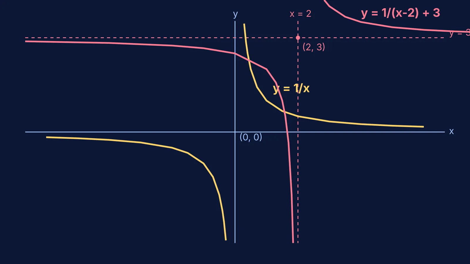
The graph of the reciprocal function y = 1/x is known as a rectangular hyperbola. It is one of the foundational curves in mathematics, introducing students to the core idea of a function that breaks into two entirely separate branches instead of forming a single continuous line.
Because you cannot mathematically divide by zero, the graph behaves in extreme ways as x approaches zero. It shoots towards infinity rather than neatly crossing the y-axis, and it flattens out towards zero as x grows infinitely large. Understanding these strict boundaries is the key to drawing it and any shifted version of it successfully.
What is the graph of y = 1/x?
Plotting the reciprocal function reveals a curve clearly divided into two unconnected parts, known as branches.
In the first quadrant, where x is positive, y is also positive. As x increases steadily (for example, taking values like 10, 100, or 1000), the value of 1/x shrinks closer and closer to zero. This is why the right side of the graph flattens out. Conversely, as x gets very close to zero from the positive side (using values like 0.1 or 0.01), y becomes extremely large. This causes the graph to shoot sharply upward.
In the third quadrant, where x is negative, y is correspondingly negative. The exact same pattern mirrors the first quadrant, but strictly with negative values. When x is −100, y is −0.01, and when x is −0.01, y drops all the way down to −100.
If tracing limits and calculating small fractions feels abstract, the Fermi Concept Library places reciprocal functions on a visual map, showing exactly how they connect to limits and calculus.
How do you find the asymptotes?
An asymptote is a line that a curve closely approaches as it heads towards infinity, but never quite touches. The standard graph of y = 1/x relies on two primary asymptotes to give it its shape:
Vertical Asymptote: Set the denominator to zero. Here, x = 0 (the y-axis) is the vertical asymptote because the function is undefined there. The curve rides alongside the y-axis but never crosses it.
Horizontal Asymptote: Look at what happens when x becomes enormously large. The fraction 1/x approaches zero, making y = 0 (the x-axis) the horizontal asymptote.
Both the domain and the range of y = 1/x include all real numbers except zero, reflecting the presence of these two boundaries.
What is origin symmetry?
The reciprocal function is an odd function, which means it exhibits origin symmetry. If you take the graph and rotate it exactly 180° around the central origin point (0,0), it lands exactly on itself.
Mathematically, an odd function satisfies the fundamental rule f(−x) = −f(x). For example, if you input x = 2, the output is 0.5. If you input x = −2, the output is −0.5. Because the points (2, 0.5) and (−2, −0.5) are exactly opposite each other across the origin, the two branches form perfect rotational mirrors. This symmetry is incredibly useful because if you know how to draw the positive branch, you can instantly trace the negative branch by simply flipping it.
How do you graph y = 1/(x − 2) + 3?
Transforming the standard hyperbola is simply a matter of moving its asymptotes. The general shift form is y = a/(x − h) + k, where h moves the entire graph horizontally and k moves it vertically.
Let's graph y = 1/(x − 2) + 3 step by step:
Find the vertical asymptote: Set the denominator to zero. Here, x − 2 = 0, so the new vertical boundary is x = 2.
Find the horizontal asymptote: Read the constant added at the end. Here, y = 3.
Draw the new axes: Sketch dashed lines at x = 2 and y = 3. These act as your new, shifted origin.
Plot a few points: Choose x-values near the vertical asymptote to shape the curves. For instance, at x = 3, y = 1/(3−2) + 3 = 4. At x = 1, y = 1/(1−2) + 3 = 2.
Sketch the branches: Draw smooth curves in the "upper-right" and "lower-left" regions created by your new dashed asymptotes.
If you prefer to see the transformation happen instantly, the Fermi Simulation Lab lets you drag sliders for h and k and watch the asymptotes slide across the grid in real time.
Learning to read horizontal and vertical shifts directly from an equation is a powerful mathematical tool. It provides a foundational understanding necessary for tackling limits at infinity of rational functions. It saves you from the tedious task of calculating a long table of values, allowing you to focus on the overall structure. Furthermore, mastering these geometric shifts gives you an instant, accurate picture of the function's boundaries, making it much easier to determine the range of a rational function without relying on complex algebra.


