Deriving the First-Order Integrated Rate Equation for Board Exams

In a first-order reaction, the rate depends on the first power of the reactant's concentration. This means if you double the concentration of the reactant, the rate of the reaction doubles. If you halve the concentration, the rate also halves. If we have a simple reaction where a single reactant R turns into a product P (written as R → P), the differential rate law is expressed in terms of a rate constant, k.

Rate = −d[R]/dt = k[R]

Here, k is the rate constant, and the negative sign shows that the reactant's concentration is falling as the reaction progresses. Its units vary depending on the reaction order. For a first-order process, you can find the units of the rate constant to be simply inverse time (s⁻¹). To find the concentration at any given time, we gather the [R] terms on one side and the time terms (t) on the other:

d[R] / [R] = −k dt

How do you derive the integrated rate equation for a first order reaction?

To find the integrated form, you integrate both sides of the differential equation from time zero to time t. This simple application of integral calculus reveals how the concentration changes smoothly over time, rather than just giving the rate at a single instant.

∫ (1/[R]) d[R] = −k ∫ dt

ln[R] = −kt + I

The letter I represents the constant of integration. To find it, we look at the start of the reaction. At time t = 0, the concentration [R] is exactly the initial concentration, [R]₀.

ln[R]₀ = −k(0) + I

I = ln[R]₀

Substitute this initial value back into the integrated equation:

ln[R] = −kt + ln[R]₀

Rearranging the terms gives the integrated rate equation in its natural logarithm form:

kt = ln[R]₀ − ln[R]

kt = ln([R]₀ / [R])

k = (1/t) ln([R]₀ / [R])

To master chemical kinetics, the Fermi Concept Library holds every concept in physics, chemistry, biology, mathematics and computing, each with its own lesson and its place in the map. It is a clear way to see how differential rate laws connect to half-life and reaction mechanisms.

How to convert the rate equation to base 10 log?

Calculations in chemistry are usually easier in base 10 because scientists routinely work with pH, pKa, and other logarithmic scales that are based on powers of ten. To convert a natural logarithm (ln, which is base e) to a common logarithm (log₁₀), you simply multiply by the conversion factor 2.303.

k = (2.303 / t) log([R]₀ / [R])

This is the standard form of the first-order integrated rate equation required in CBSE and state board exams. The rate constant k itself depends heavily on temperature, a relationship measured by the temperature coefficient of the reaction rate.

How to calculate the half-life of a first order reaction?

The half-life (t½) is the time it takes for the reactant concentration to drop to exactly half of its starting value. At t = t½, the concentration [R] = [R]₀ / 2.

Substitute these values into the base-10 rate equation:

k = (2.303 / t½) log([R]₀ / ([R]₀ / 2))

k = (2.303 / t½) log(2)

Because the logarithm of 2 is roughly 0.3010, the numerator becomes 2.303 × 0.3010 = 0.693.

t½ = 0.693 / k

Notice that [R]₀ has completely vanished from the final equation. The half-life of a first-order reaction is completely independent of the starting concentration. According to the principles of radiometric dating, radioactive decay strictly follows first-order kinetics. A radioactive sample takes the exact same amount of time to decay from 100 grams to 50 grams as it does to decay from 10 grams to 5 grams, or from 1 gram to 0.5 grams. This constant half-life is why scientists use first-order kinetics to reliably date ancient rocks and fossils.

What do the graphs for a first-order reaction look like?

Board exams frequently ask you to identify a reaction's order directly from its graph. Visualizing the data is often the quickest way to solve these problems.

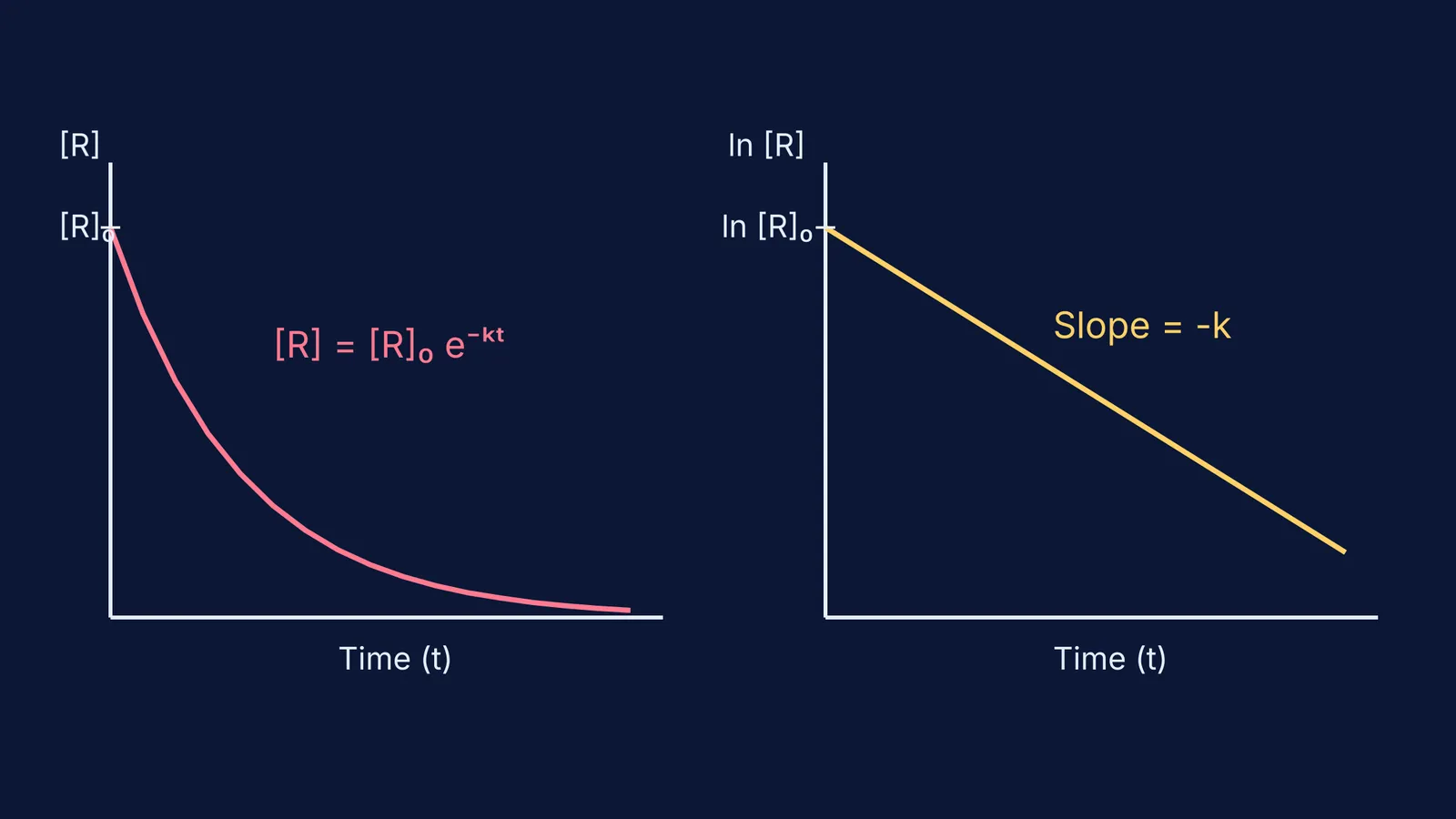
The equation ln[R] = −kt + ln[R]₀ is a straight line in the form y = mx + c. If you plot ln[R] against time t, you get a downward-sloping straight line. Its slope is −k, and it meets the y-axis at ln[R]₀. This matches the strict rules for reading integrated rate law graphs, where finding the straight-line plot tells you the order of the reaction.

If you plot log[R] instead of the natural log, the line is still perfectly straight, but its slope becomes −k/2.303. If you plot the concentration [R] against time directly, you get an exponential decay curve that approaches zero but never mathematically touches it.

If you are getting tangled in the calculus of these equations, Fermi's AI tutor can help. It works out what you already know, builds a plan for the session, and teaches through it — checking understanding as it goes.