

On this page
In differential calculus, finding where a curve peaks or bottoms out starts with its slope. The first derivative test is a systematic way to classify these turning points by observing how the slope behaves around them.
How do you find the critical points?
A local maximum or minimum can only occur at a critical point. According to OpenStax Calculus/04%3A_Applications_of_Derivatives/4.03%3A_Maxima_and_Minima), a point c in the domain of f is a critical point if the derivative f′(c) = 0 or if f′(c) is undefined. At these points, the tangent line to the curve is either perfectly horizontal, or the curve has a sharp corner or vertical tangent.
Finding these points is the first step. You calculate the derivative f′(x) and solve the equation f′(x) = 0. You must also check for any values of x in the domain where f′(x) does not exist.
If you get stuck finding a difficult derivative or factoring the resulting polynomial, the Fermi Problem Library has worked problems with a step-by-step solver that explains the reasoning rather than printing an answer.
How do you apply the first derivative test?
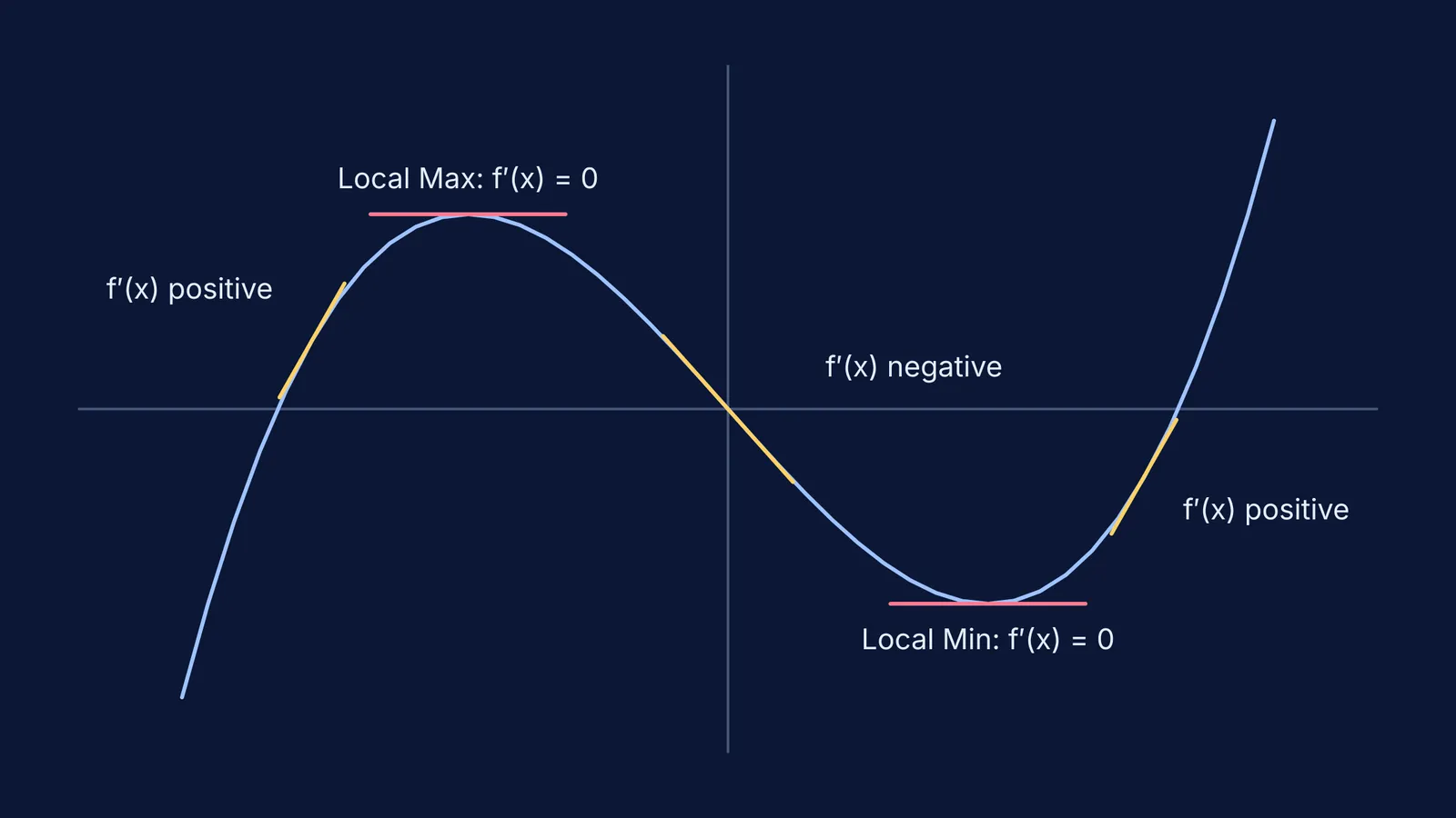
Once you have identified a critical point c, you need to test the sign of the first derivative on the intervals immediately to its left and right. This tells you whether the function is increasing or decreasing before and after the point.
According to OpenStax Calculus/04%3A_Applications_of_Derivatives/4.05%3A_Derivatives_and_the_Shape_of_a_Graph), the first derivative test rules are:
Local Maximum: If f′(x) changes from positive to negative (the curve goes up, then down), there is a local maximum at c.
Local Minimum: If f′(x) changes from negative to positive (the curve goes down, then up), there is a local minimum at c.
What if the sign does not change?
A zero derivative does not guarantee a maximum or minimum. If f′(x) has the same sign on both sides of a critical point, the function continues in its original direction.
For example, for f(x) = x³, the derivative f′(x) = 3x² is zero at x = 0. However, the sign of f′(x) is positive for both x < 0 and x > 0. Since there is no sign change, x = 0 is neither a local maximum nor a local minimum. It is simply a point where the curve momentarily flattens out before continuing to rise.
How do you handle an undefined derivative?
The first derivative test still works perfectly when the derivative is undefined, as long as the original function is continuous at that point.
Consider the absolute value function, f(x) = |x|. The graph forms a sharp "V" shape at the origin. The derivative f′(x) is −1 for all x < 0, and f′(x) is 1 for all x > 0. At exactly x = 0, the derivative is undefined because the left-hand and right-hand limits of the difference quotient do not match.
However, x = 0 is still a critical point. By applying the test, we see that f′(x) changes from negative to positive around x = 0. Therefore, the function has a local minimum at x = 0. This shows why we must always include points where f′(x) is undefined in our list of critical points.
A worked example: f(x) = x³ − 3x² − 9x − 1
Let us classify the critical points for the function f(x) = x³ − 3x² − 9x − 1.
Find the derivative: We differentiate the polynomial term by term to get f′(x) = 3x² − 6x − 9.
Find critical points: We set f′(x) = 0 and factor out the common term to get 3(x² − 2x − 3) = 0, which factors further to 3(x − 3)(x + 1) = 0. The critical points are x = −1 and x = 3. The derivative is a polynomial, so it is never undefined.
Test the intervals: We divide the number line into three sections: x < −1, −1 < x < 3, and x > 3.
For x < −1, choose x = −2: f′(−2) = 3(−5)(−1) = 15, which is positive.
For −1 < x < 3, choose x = 0: f′(0) = 3(−3)(1) = −9, which is negative.
For x > 3, choose x = 4: f′(4) = 3(1)(5) = 15, which is positive.
Conclusion: At x = −1, the sign changes from positive to negative, making it a local maximum. At x = 3, the sign changes from negative to positive, making it a local minimum.
If you struggle to picture why a zero slope can fail to be an extremum or what an undefined derivative looks like, you can explore the graphs of these cases interactively in the Fermi Concept Library, which covers every concept in mathematics, each with its own lesson.


