

On this page
When you plot an exponential function of the form y = aˣ, the shape of the curve depends entirely on the value of the base a. If the base is greater than 1, the numbers multiply repeatedly by a large factor, causing the graph to climb steeply towards infinity. But what happens to the graph of a power x when a is less than 1?
How does the graph of a power x change when a is less than 1?
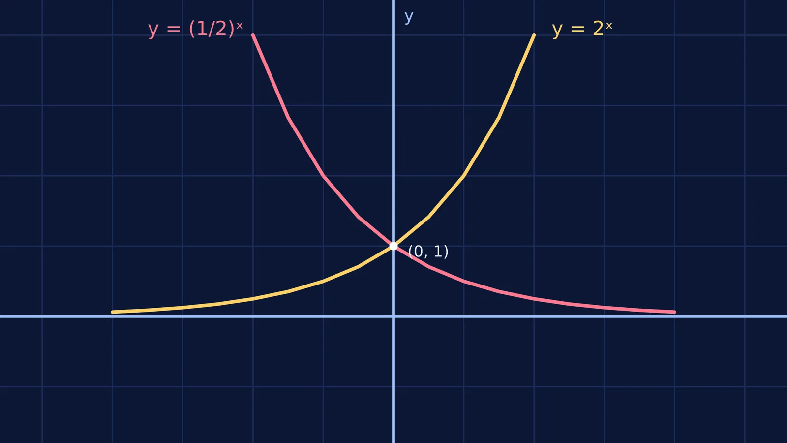
When the base a is strictly between 0 and 1, the function describes exponential decay. Instead of rising, the graph is strictly decreasing as you move your eyes from left to right. According to the OpenStax Algebra and Trigonometry/06%3A_Exponential_and_Logarithmic_Functions/6.02%3A_Graphs_of_Exponential_Functions) textbook, an exponential function where 0 < a < 1 has a domain of all real numbers and a range of all positive real numbers.
The reason for this drop lies in the mechanics of fractions. As x becomes a larger positive number, you are multiplying a fraction by itself. Because taking a fraction of a fraction results in an even smaller number, the y-value shrinks continuously. The curve flattens out and approaches the x-axis, meaning the x-axis (y = 0) acts as a horizontal asymptote on the right side of the graph. The curve gets closer and closer to zero but never actually touches or crosses the axis, because no positive fraction raised to a real power can ever truly reach zero. On the far left side, however, raising a proper fraction to a large negative power results in a massive positive number, which is why the curve shoots upwards toward positive infinity.
The shared intercept at (0, 1)
Whether the base is 2, 10, or 1/2, one defining point never changes. Every parent exponential function passes exactly through the y-intercept at the coordinate (0, 1). This mathematical constant occurs because any non-zero real number raised to the power of 0 equals exactly 1. If you are ever unsure where to start your sketch on a blank page, plotting the point (0, 1) immediately grounds the rest of the curve and gives you a reliable anchor.
Why do graphs of base a and 1/a reflect across the y-axis?
The graphs of y = 2ˣ and y = (1/2)ˣ are exact mirror images of each other, reflecting perfectly across the y-axis.
Because of the algebraic rules governing negative exponents, the expression (1/a)ˣ is structurally equivalent to a⁻ˣ. In coordinate geometry, multiplying the input x by −1 reflects any given graph horizontally across the vertical y-axis. Therefore, if the coordinate point (2, 4) sits safely on the curve of y = 2ˣ, its exact mirror point (−2, 4) sits perfectly on the curve of y = (1/2)ˣ. This symmetry is useful when checking your work.
How to sketch an exponential decay graph in an exam
If you are asked to draw an exponential graph with a base less than 1 under exam conditions, you should follow a consistent mechanical sequence to lock in the marks efficiently.
Draw the asymptote: Begin by sketching a light dashed line directly along the x-axis (where y = 0) to clearly show the lower boundary of the range.
Mark the intercept: Plot and label the point at (0, 1) on the y-axis, making sure it is distinctly visible to the examiner.
Plot the reference points: Pick two easy input values to give your curve structure. Substitute x = 1 to find the point (1, a). Then substitute x = −1 to find the point (−1, 1/a). For example, if your equation is y = (1/3)ˣ, your reference points will be (1, 1/3) and (−1, 3).
Draw the continuous curve: Connect your three points with a single, smooth curve that drops steeply from the top left quadrant, passes through the reference points, and sweeps out gently along the horizontal asymptote to the far right.
If you have concept gaps around how changing the numerical base stretches or squashes these curves, the Fermi Concept Library maps every concept in mathematics, each with its own lesson. Visualising the difference between exponential growth and decay makes solving complex inequalities and domain-range problems much easier. You can apply similar coordinate logic when analysing Population growth and cooling: exponential models via dy/dt = ky, or when evaluating the Range of a rational function using the discriminant method.


