

On this page
When an unstable atomic nucleus can transition into more than one final state, it does not pick a pathway after waiting; instead, multiple decay mechanisms compete continuously. For example, a heavy nucleus might undergo alpha emission to form one element or beta decay to form another. The IUPAC Compendium of Chemical Terminology defines the decay constant λ as the transition probability per unit time for a single nucleus. When two distinct decay mechanisms—say, process 1 with decay constant λ₁ and process 2 with decay constant λ₂—operate independently on the same nucleus, the overall probability per unit time that the nucleus disintegrates is simply the sum of the two probabilities:
λ = λ₁ + λ₂
In a sample containing N undecayed parent nuclei at time t, the rate of loss due to the first pathway is −(dN/dt)₁ = λ₁ N, and the rate of loss due to the second pathway is −(dN/dt)₂ = λ₂ N. Because both pathways deplete the same parent population simultaneously, the total rate of disintegration is:
−dN/dt = (λ₁ + λ₂) N = λ N
Integrating this first-order rate equation gives N(t) = N₀ e^(−λ t), where N₀ is the initial number of nuclei. As discussed in our guide to radioactive decay and half-life, the overall population decays exponentially, governed not by either individual pathway alone, but by the combined decay constant λ.
Why do decay constants add when a nucleus has two decay modes?
Because decay events in radioactive nuclei are memoryless stochastic processes, the probability of decaying through channel 1 within a short time interval dt is λ₁ dt, and the probability of decaying through channel 2 is λ₂ dt. Because these decay channels are mutually exclusive—a single nucleus cannot simultaneously emit an alpha particle and a beta particle in the same primary transition—their probabilities add directly:
P(decay in dt) = (λ₁ + λ₂) dt = λ dt
This simple addition explains why the decay constant of the parent nuclide increases whenever an alternative decay mode exists. The parent nucleus does not slow down one channel to accommodate another; each channel draws from the available pool at its own inherent rate.
How do you calculate the effective half-life from partial half-lives?
A common mistake in physics tests is trying to average the two individual half-lives. As codified in the IUPAC Gold Book, half-life T is inversely related to the decay constant through T = ln 2 / λ; hence, larger decay constants produce shorter half-lives. Substituting λ = ln 2 / T, λ₁ = ln 2 / T₁, and λ₂ = ln 2 / T₂ into the additive decay constant relation yields:
(ln 2) / T = (ln 2) / T₁ + (ln 2) / T₂
Dividing every term by ln 2 produces the reciprocal rule for effective half-life:
1/T = 1/T₁ + 1/T₂
For two competing decay pathways, cross-multiplying gives:
T = (T₁ × T₂) / (T₁ + T₂)
This relationship is mathematically identical to finding the equivalent resistance of two parallel resistors. Because the sum 1/T₁ + 1/T₂ is strictly greater than either individual term, the effective half-life T is always shorter than both T₁ and T₂. Adding an extra exit route always empties the parent container faster.
How do you find the fraction and yield of each daughter product?
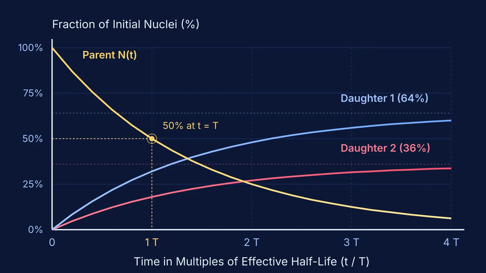
The IUPAC Gold Book defines the branching fraction as the fraction of decaying nuclei that disintegrate along a specified channel. Because the production rate of daughter nuclide 1 is dN₁/dt = λ₁ N(t) and daughter nuclide 2 is dN₂/dt = λ₂ N(t), the ratio of production rates is constant at every moment:
(dN₁/dt) / (dN₂/dt) = λ₁ / λ₂ = T₂ / T₁
Notice the reciprocal flip: the faster mode has the larger decay constant and the shorter partial half-life, producing a correspondingly larger share of daughter nuclei. Integrating both rates from t = 0 gives the branching fractions f₁ and f₂:
f₁ = λ₁ / (λ₁ + λ₂) = T₂ / (T₁ + T₂)
f₂ = λ₂ / (λ₁ + λ₂) = T₁ / (T₁ + T₂)
Real radioisotopes exhibit this branching behavior. Evaluated nuclear data from the Brookhaven National Laboratory NuDat 3 database records that Bismuth-212 (²¹²Bi) has a total half-life of 60.55 minutes. It undergoes beta-minus decay 64.06% of the time to form Polonium-212 and alpha decay 35.94% of the time to form Thallium-208. Using the branching relation, its partial half-life for beta decay alone is 60.55 / 0.6406 ≈ 94.52 minutes, while its partial half-life for alpha decay alone is 60.55 / 0.3594 ≈ 168.48 minutes. Just as in our analysis of counting alpha and beta decays in a radioactive series, both pathways feed into the decay chain at predictable, constant fractions.
What does a worked branched decay problem look like?
Problems on branched decay frequently appear in competitive examinations like JEE Main, conducted by the National Testing Agency. Working through them systematically requires three clear steps:
Express all half-lives in matching time units. Suppose a parent nucleus decays by alpha emission with partial half-life T₁ = 12 minutes and beta emission with partial half-life T₂ = 24 minutes.
Calculate effective half-life using the reciprocal sum: 1/T = 1/12 + 1/24 = 3/24 = 1/8, so T = 8 minutes.
Compute the branching fractions: f₁ = 24 / (12 + 24) = 2/3 (66.67%), and f₂ = 12 / (12 + 24) = 1/3 (33.33%).
If you begin with 1.2 × 10¹² undecayed nuclei, after 24 minutes (exactly 3 effective half-lives), the remaining parent count is N = N₀ / 2³ = 1.5 × 10¹¹ nuclei. That means 1.05 × 10¹² nuclei have decayed. The number of alpha daughter nuclei formed is (2/3) × 1.05 × 10¹² = 7.0 × 10¹¹ nuclei, while the beta daughter count is (1/3) × 1.05 × 10¹² = 3.5 × 10¹¹ nuclei. As expected from first-order kinetics in chemical kinetics rate laws, the ratio of the two products remains exactly 2:1 at all times.
Setting up the reciprocal equation correctly and converting time units before adding prevents the standard algebraic traps that catch students in exam halls. The Fermi Problem Library has worked problems with a step-by-step solver that explains the reasoning rather than printing an answer. To review the underlying theory across atomic and modern physics, the Fermi Concept Library covers every concept in physics, chemistry, biology, mathematics and computing, each with its own lesson and its place in the map.


