

On this page
Many curve-sketching mistakes are not calculus mistakes. They are order mistakes: a student finds f′ first, gets a turning point outside the domain, and draws a hump through an asymptote. A fixed order stops that.
OpenStax Calculus Volume 1, a free textbook, gives a six-step problem-solving strategy for drawing the graph of a function: domain, x- and y-intercepts, end behaviour as x goes to plus and minus infinity, vertical asymptotes, f′ for increasing and decreasing intervals, and f″ for concavity. We add one quick check, symmetry, after the domain, because it can halve the work.
What is the order of steps for curve sketching?
Domain. Write down every excluded point; each is a candidate vertical asymptote or hole.
Symmetry. Work out f(−x). In OpenStax's definition of even and odd functions, an even function satisfies f(−x) = f(x) and is symmetric about the y-axis, and an odd function satisfies f(−x) = −f(x) and is symmetric about the origin.
Intercepts. Find f(0), if defined, and solve f(x) = 0.
Asymptotes. A line y = L is a horizontal asymptote if f(x) tends to L as x tends to plus or minus infinity. A vertical asymptote x = a is where f(x) shoots off to plus or minus infinity as x approaches a from at least one side.
Monotonicity. Find f′, its zeros and where it is undefined, then make a sign chart. Where f′ > 0 the curve rises; where f′ < 0 it falls.
Concavity. Find f″ and make a second sign chart. By the test for concavity, f is concave up where f″ > 0 and concave down where f″ < 0; a point where f is continuous and concavity changes is an inflection point.
Only then draw: asymptotes dashed first, then the special points, then pieces that follow both sign charts. If step 5 is where you get stuck, our guide to increasing and decreasing functions using the sign of f′ builds the sign chart slowly.
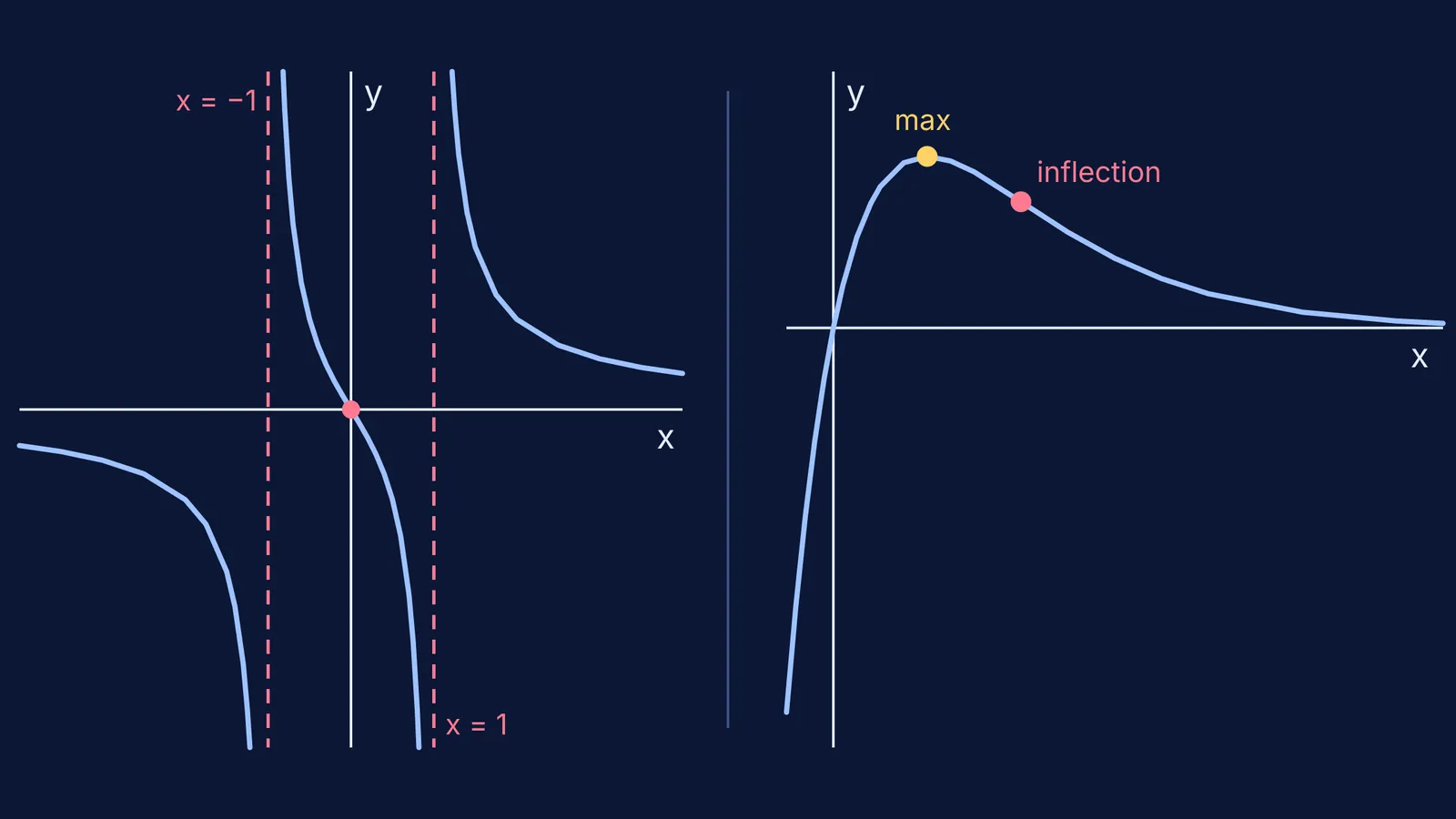
How do you sketch a rational function like 2x/(x² − 1)?
Domain: x² − 1 ≠ 0, so x ≠ 1 and x ≠ −1.
Symmetry: f(−x) = −f(x), so f is odd and symmetric about the origin. Sketch the right half and rotate it.
Intercepts: f(x) = 0 only at x = 0, so the only intercept is the origin.
Asymptotes: the numerator has lower degree than the denominator, so f(x) tends to 0 at both ends and y = 0 is a horizontal asymptote (see limits at infinity of rational functions). At x = 1 and x = −1 the denominator is zero and the numerator is not, so both are vertical asymptotes.
Monotonicity: f′(x) = −2(x² + 1)/(x² − 1)². The top is always negative and the bottom positive, so f falls on every piece and has no maximum or minimum.
Concavity: f″(x) = 4x(x² + 3)/(x² − 1)³. Concave down for x < −1, up for −1 < x < 0, down for 0 < x < 1, up for x > 1. Concavity changes at x = 0 and f is continuous there, so the origin is an inflection point.
The sketch: three falling pieces. The middle one drops from plus infinity near x = −1, through the origin, to minus infinity near x = 1.
How do you sketch an exponential function like xe^(−x)?
Domain: all real numbers.
Symmetry: f(−x) = −xe^x, which is neither f(x) nor −f(x). No symmetry.
Intercepts: e^(−x) is never zero, so f(x) = 0 only at x = 0. The only intercept is the origin.
Asymptotes: e^x grows faster than x, so xe^(−x) tends to 0 as x tends to plus infinity: y = 0 is a horizontal asymptote on the right only. On the left f(x) tends to minus infinity. No vertical asymptotes.
Monotonicity: f′(x) = e^(−x)(1 − x). Rising for x < 1, falling for x > 1. By the first derivative test, f′ changing from positive to negative makes x = 1 a local maximum, at height 1/e, about 0.37.
Concavity: f″(x) = e^(−x)(x − 2). Concave down for x < 2, up for x > 2. The inflection point is (2, 2/e²), about (2, 0.27).
The sketch: up through the origin to a peak at (1, 0.37), changing bend at (2, 0.27), then flattening towards the x-axis.
What mistakes cost marks in curve sketching?
Plotting a turning point at an excluded x-value. Domain first prevents it.
Forgetting that signs can change at a vertical asymptote. Put excluded points on every sign chart.
Calling any point with f″ = 0 an inflection point. Check that concavity changes there.
Drawing a curve across a vertical asymptote, where f is not defined.
Curve sketching feeds straight into finding maxima and minima in applied problems. To practise the six steps on more functions, the Fermi Problem Library has worked problems with a step-by-step solver that explains the reasoning rather than printing an answer, so you can see where your own sign chart went wrong.