

On this page
Why is mutual inductance bounded by the square root of L₁L₂?
When two coils are placed near one another, a changing current in the first induces an electromotive force in the second. The strength of this interaction is quantified by mutual inductance M, measured in henries (H). In physics and engineering exams like JEE Advanced, a common question is whether M can take any value if turns are increased. In reality, mutual inductance is strictly bounded by the self-inductances L₁ and L₂ through M ≤ √(L₁L₂).
The theoretical origin of this bound comes from energy conservation. As Richard Feynman demonstrates in *The Feynman Lectures on Physics* (Vol. II, Chapter 17, Section 17-8), the total magnetic energy U stored in two coupled coils carrying currents I₁ and I₂ is U = (1/2) L₁ I₁² + (1/2) L₂ I₂² ± M I₁ I₂. Because magnetic field energy density is everywhere proportional to B² / (2μ₀), total stored energy U must remain non-negative for every possible current combination.
Requiring U ≥ 0 for all real currents demands that the discriminant of the quadratic form satisfy (±M)² − 4(1/2 L₁)(1/2 L₂) ≤ 0, which simplifies directly to M² ≤ L₁ L₂ or |M| ≤ √(L₁L₂).
The coupling coefficient k is defined as the dimensionless ratio k = M / √(L₁L₂), which is physically restricted to 0 ≤ k ≤ 1 by energy conservation (The Feynman Lectures on Physics). If k exceeded 1, one could supply opposing currents and extract net work from negative magnetic energy. To see how energy is stored in a single coil, read our guide on self and mutual inductance.
How do coil spacing and orientation change the coupling coefficient?
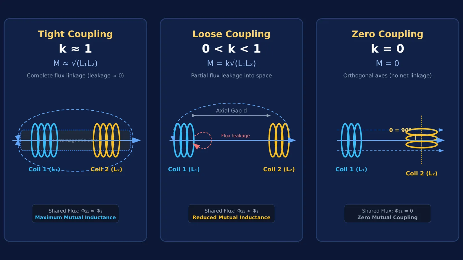
From a geometric viewpoint, the coupling coefficient k measures the fraction of magnetic flux produced by one coil that links the turns of the other (OpenStax University Physics). If coil 1 directs a flux fraction k₁ through coil 2, and coil 2 directs k₂ through coil 1, reciprocity establishes that k = √(k₁ k₂).
Three physical factors determine k:
Axial spacing: As the separation d between coils increases, magnetic flux leaks into surrounding air rather than linking the second coil, driving k toward 0.
Angular orientation: Magnetic flux through a loop equals Φ = B · A = B A cos θ. For concentric circular coils, mutual inductance varies as M(θ) = M₀ cos θ, where θ is the angle between their magnetic axes (IEEE Transactions on Magnetics). When coils are perpendicular (θ = 90°), no net flux links the windings, producing k = 0.
Core permeability: Winding coils on a high-permeability ferromagnetic core channels flux through both coils, lifting k to between 0.95 and 0.99 in transformers compared to 0.1 to 0.5 in air-core coils (OpenStax University Physics).
In the NCERT Class 12 Physics textbook (Chapter 6, Section 6.10.1), two long coaxial solenoids have mutual inductance M = μ₀ n₁ n₂ π r₁² l. When both solenoids share the same radius, this formula simplifies to M = √(L₁L₂), giving ideal coupling k = 1. To see how solenoid geometry governs magnetic fields, explore our explainers on Biot-Savart and Ampère's law and circulating electric fields inside a solenoid.
How do you solve coupled inductor problems in JEE and NEET?
Coupled inductor numericals in competitive examinations like JEE Main and NEET-UG follow the series-combination rules derived from Faraday's law (OpenStax University Physics), asking you to find M or the equivalent inductance of two coils connected in series.
Suppose Coil 1 has L₁ = 40 mH and Coil 2 has L₂ = 90 mH, with coupling coefficient k = 0.75.
First, calculate the maximum possible mutual inductance: M_max = √(L₁ L₂) = √(40 mH × 90 mH) = 60 mH.
Next, find the actual mutual inductance: M = k √(L₁ L₂) = 0.75 × 60 mH = 45 mH.
When connected in series, total inductance depends on terminal polarities:
Series aiding: L_eq = L₁ + L₂ + 2M = 40 + 90 + 2(45) = 220 mH.
Series opposing: L_eq = L₁ + L₂ − 2M = 40 + 90 − 2(45) = 40 mH.
How do engineers control the coupling coefficient in practical circuits?
Circuit designers select coil orientations and spacing to maximize energy transfer or prevent electromagnetic cross-talk, applying coupling principles analyzed by Kim and Lee in the *Journal of Electromagnetic Engineering and Science*:
Tight coupling (k ≈ 0.95 to 0.99): Achieved using a closed high-permeability ferromagnetic core or interleaved windings, as described in OpenStax University Physics. This geometry confines magnetic flux and minimizes leakage inductance in power transformers.
Loose to moderate coupling (k ≈ 0.10 to 0.50): Position air-core coils with an intentional separation distance d. This configuration is widely used in wireless power transfer and resonant band-pass circuits where loose coupling allows sharp resonant tuning.
Zero coupling (k = 0): Mount adjacent coils at right angles (θ = 90°) or place them at geometric null positions where opposing fluxes cancel. Circuit board layouts use orthogonal inductor orientations to prevent stray magnetic coupling and signal interference.
When working through multi-concept numericals, the Fermi Problem Library provides worked problems with a step-by-step solver that explains the reasoning rather than printing an answer. To review how magnetic induction connects with alternating currents, browse the lessons in the Fermi Concept Library.


