

On this page
When applying Gauss's law in electrostatics, students often encounter a puzzling factor of 2. An infinite, non-conducting sheet of uniform surface charge density σ produces an electric field of E = σ / 2ε₀. Yet just outside the surface of a charged conductor with that same local density σ, the electric field is E = σ / ε₀.
Why does the conductor produce double the field strength of an isolated sheet? According to OpenStax University Physics, the answer comes down to boundary conditions and flux paths. Inside a conductor in electrostatic equilibrium, mobile charges rearrange until the interior electric field is zero, which alters how electric flux exits the surface.
Why is the electric field near a non-conducting sheet σ / 2ε₀?
Imagine an ideal, infinite, non-conducting plane carrying a uniform positive surface charge density σ. Because the sheet is an insulator, charges remain fixed throughout its geometry. Planar symmetry requires that the electric field lines point perpendicularly away from the sheet on both sides, with equal magnitude at any given distance.
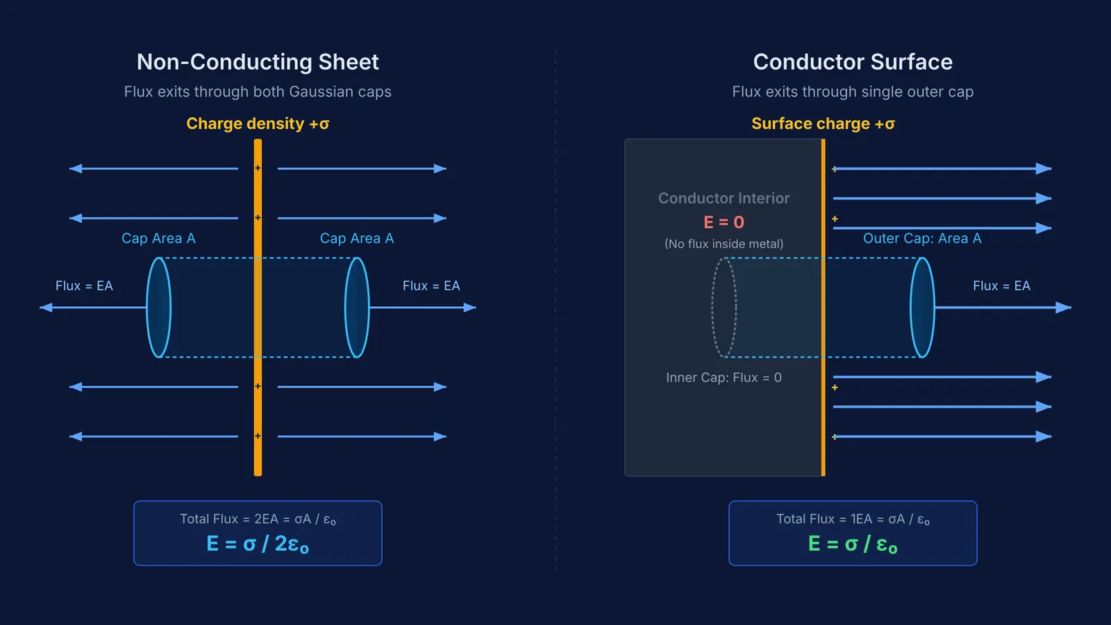
To calculate the field strength, consider a cylindrical Gaussian surface—commonly called a pillbox—oriented with its axis perpendicular to the sheet. The cylinder's two flat end caps, each with cross-sectional area A, lie parallel to the sheet on opposite sides. Because the electric field is parallel to the cylinder's curved side walls, zero electric flux passes through the sides.
Flux leaves exclusively through the two end caps. Since the field points outward on both sides, the total electric flux is Φ = EA + EA = 2EA. The total charge enclosed inside the cylinder is q_enc = σA. Applying Gauss's law gives 2EA = σA / ε₀.
Dividing both sides by 2A yields E = σ / 2ε₀. The electric flux splits equally in two opposite directions. As explained in HyperPhysics, the resulting electric field of an isolated sheet is exactly half that of a conductor in equilibrium with the same surface charge density.
Why is the electric field just outside a conductor σ / ε₀?
Now replace the non-conducting sheet with a thick conducting slab carrying surface charge density σ. Conductors contain mobile conduction electrons. In electrostatic equilibrium, these charges redistribute across the outer boundary until the net electric field anywhere inside the metal is zero (E = 0).
Construct a Gaussian pillbox across the conductor's outer boundary. One flat cap of area A is positioned just outside the surface in air or vacuum. The other cap is buried within the interior of the metal slab. The cylindrical walls cut perpendicularly through the surface.
Because the electric field inside a conductor is zero, no flux passes through the inner cap. Furthermore, the field just outside a conductor must be strictly perpendicular to the surface; any parallel component would accelerate surface electrons, violating equilibrium. Consequently, no flux crosses the cylinder's side walls either.
All the electric flux from the enclosed charge q_enc = σA is forced out through the single exterior cap. Setting up Gauss's law gives 1EA = σA / ε₀.
As demonstrated in OpenStax University Physics, eliminating the interior flux path directs all outward flux into the exterior space, producing double the field of a two-sided sheet for the same local charge density: E = σ / ε₀.
Field near conductor σ / ε₀ vs sheet σ / 2ε₀: how does superposition explain the factor of 2?
Counting Gaussian caps provides a straightforward mathematical proof, but the physical mechanism behind this result is explained by the principle of superposition. To see how, split the total surface charge of the conductor into two parts: a tiny patch directly beneath the observation point, and all the remaining charges across the rest of the conductor.
A tiny, flat surface patch of charge density σ acts locally like a small sheet of charge. Very close to the surface, this patch produces a field of magnitude σ / 2ε₀ directed outward into space and σ / 2ε₀ directed inward into the conductor.
For the total internal field to remain zero in electrostatic equilibrium, all the other charges on the conductor must generate an opposing field of exactly σ / 2ε₀ pointing outward at that same location. This internal field from the rest of the conductor cancels the patch's inward field, leaving E_net = 0 inside the bulk metal.
Just outside the surface, the field from the rest of the conductor continues in the outward direction with that same magnitude σ / 2ε₀. Here, the patch's outward field and the rest of the conductor's outward field reinforce each other:
E_net = σ / 2ε₀ + σ / 2ε₀ = σ / ε₀
The superposition view reveals that the conductor's surface field reaches σ / ε₀ because the remaining charges on the conductor set up an additional field of σ / 2ε₀ that cancels the patch inside and reinforces it outside.
How does this distinction apply to parallel plate capacitors?
This factor of 2 often causes errors in parallel-plate capacitor problems. Consider two parallel conducting plates given equal and opposite total charges +Q and -Q. Because opposite charges attract, all excess charge migrates to the inner facing surfaces, establishing an inner surface charge density of +σ on one plate and -σ on the other.
You can determine the uniform field between the plates using two different but equivalent methods:
The Conductor Approach: Looking directly at the inner surface of the positive conducting plate, it is a conductor surface with local charge density σ. The field just outside its face is E = σ / ε₀.
The Sheet Approach: Treat the two charged layers as independent sheets of charge. The positive layer produces an electric field of σ / 2ε₀ pointing away from it toward the negative plate. The negative layer produces a field of σ / 2ε₀ pointing toward itself. Between the plates, both fields point in the same direction, summing to σ / 2ε₀ + σ / 2ε₀ = σ / ε₀. Outside the plates, the fields oppose each other and cancel to zero.
Both perspectives yield the exact same physical result. When analyzing complex field geometries, Fermi's AI tutor can work out what you already know and teach through the derivation step by step, drawing the figure and checking understanding as it goes. You can also explore connected derivations, such as setting up Gauss's law for a sphere with non-uniform charge density, in the Fermi Concept Library, which covers every concept in physics with its own lesson and its place in the map.
Once you establish the field strength between charged boundaries, you can determine related electrostatic quantities, such as calculating the energy density in an electric field or finding E from V along the potential gradient. Knowing whether flux escapes from one surface or two ensures you never lose a factor of 2.


