

On this page
In traditional titrations, we rely on indicators to change colour at the equivalence point. But what if the solution is already dark, turbid, or the acid is too weak to produce a sharp pH jump? This is where conductometric titration comes in.
Instead of watching for a colour change, we measure the electrical conductance of the solution as the titrant is added. Because different ions carry charge at different speeds, the changing composition of the mixture creates distinct straight-line graphs. The endpoint is simply the point where these lines intersect. To master these graphs, you can explore the Fermi Concept Library, which breaks down the principles of ionic mobility step by step.
Why does titrating a strong acid and strong base give a V-shaped curve?
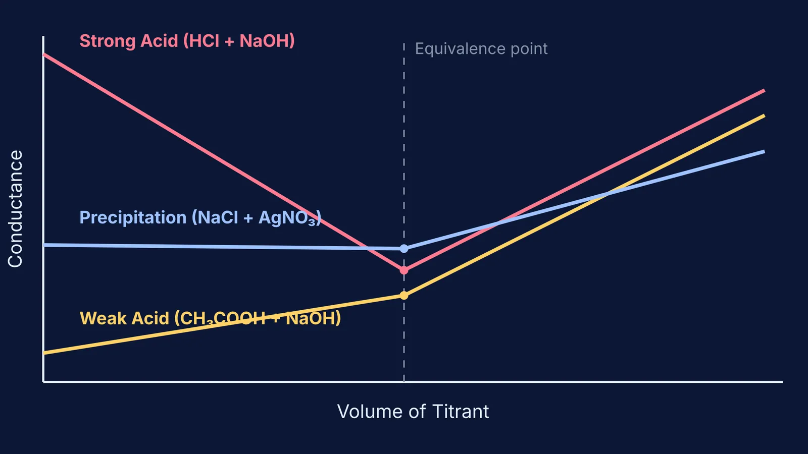
If you titrate hydrochloric acid (HCl) with sodium hydroxide (NaOH), the conductance drops steeply and then rises just as sharply. This classic V-shape is entirely due to the changing cast of ions in the beaker.
Before any base is added, the solution is highly conductive. This is because hydrogen ions (H⁺) have an exceptionally high ionic mobility—much higher than almost any other ion. As you drip NaOH from the burette, the H⁺ ions react with OH⁻ to form neutral water. Meanwhile, the H⁺ ions are replaced in the solution by sodium ions (Na⁺).
Because Na⁺ ions are much slower than H⁺ ions, the total ability of the solution to carry a current drops steadily. This forms the falling branch of the curve.
At the equivalence point, all the acid has been neutralised. The solution contains only Na⁺ and Cl⁻ ions, giving it the lowest conductance of the entire experiment.
Once you pass the equivalence point, every extra drop of NaOH adds excess Na⁺ and OH⁻ ions to the mixture. Hydroxide (OH⁻) is the second most mobile ion in aqueous chemistry. The sudden surplus of these fast-moving ions causes the conductance to climb rapidly, forming the rising branch of the V.
What happens when titrating a weak acid and a strong base?
When you titrate a weak acid like acetic acid (CH₃COOH) with a strong base like NaOH, the curve looks completely different. You can compare this to standard pH graphs in our guide to acid-base titration curves.
Initially, the conductance is very low because acetic acid is a weak electrolyte and barely dissociates into ions.
As you add NaOH, it reacts with the acid to form sodium acetate (CH₃COONa). Unlike the weak acid, this salt is highly ionised. Even though the common ion effect suppresses the dissociation of the remaining acid, the sheer number of Na⁺ and CH₃COO⁻ ions being generated causes the conductance to rise gradually.
After the equivalence point, the acid is entirely consumed. Further addition of NaOH floods the solution with highly mobile OH⁻ ions. Just as in the strong acid case, the conductance shoots up steeply. The equivalence point is found by extending the shallow pre-equivalence line and the steep post-equivalence line until they meet.
How do precipitation titrations work?
Conductometry is also brilliant for precipitation reactions, such as titrating sodium chloride (NaCl) with silver nitrate (AgNO₃). The rule here is simple: watch which ion is swapping out for which.
In the flask, you start with Na⁺ and Cl⁻. As AgNO₃ is added, the silver ions react with the chloride ions to form a solid, insoluble precipitate of AgCl, which drops out of the solution and no longer carries a current.
For every Cl⁻ ion lost, a nitrate ion (NO₃⁻) takes its place in the dissolved mixture. Because Cl⁻ and NO₃⁻ have very similar ionic mobilities, the overall conductance stays almost perfectly flat, or drops only slightly, until all the chloride is gone. (For a deeper look at how ions carry current, see our post on Molar conductivity and Kohlrausch's law).
Once the equivalence point is passed, the excess AgNO₃ adds both Ag⁺ and NO₃⁻ ions to the solution. The total ion concentration rises, and the conductance climbs steadily.
If you find yourself stuck on exam questions about equivalent concepts or calculating unknown concentrations when standard methods fail, trying a back titration might be the answer. For more practice on setting up these calculations and finding the intersection points of these graphs, try working through the exercises in the Fermi Problem Library.


