

On this page
Finding the centre of mass of a uniform rod is straightforward: it sits exactly in the middle. But in physics exams such as JEE and NEET, you are often asked about non-uniform rods where the density changes along their length. Because the mass is not spread evenly, you cannot simply pick the midpoint. To find the balance point of a non-uniform rod, you have to use integration to account for every infinitesimally small slice of mass.
This guide walks you through the general formula and the two most common density functions seen in physics problems: a density that is directly proportional to distance (λ = kx) and a density with a constant offset (λ = a + bx).
What is the formula for the centre of mass of a non-uniform rod?
For a continuous distribution of matter in one dimension, the position of the centre of mass (X_cm) is the integral of position multiplied by mass density, divided by the total mass.
The formula is: X_cm = (∫ x λ(x) dx) / (∫ λ(x) dx)
Here, λ(x) is the linear mass density (which is mass per unit length) at position x. If the rod lies along the x-axis from x = 0 to x = L, those become your limits of integration. The denominator of the formula, ∫ λ(x) dx, simply gives the total mass M of the rod. Source: Wikipedia
To understand this physically, imagine cutting the rod into tiny slices of width dx. The mass of one slice is dm = λ(x) dx. The formula is essentially summing up (x · dm) for every slice and dividing by the sum of all the dm slices. If you are struggling to picture why we split objects into elements before integrating, the Fermi Concept Library breaks down the calculus behind continuous mass distributions with clear visual steps.
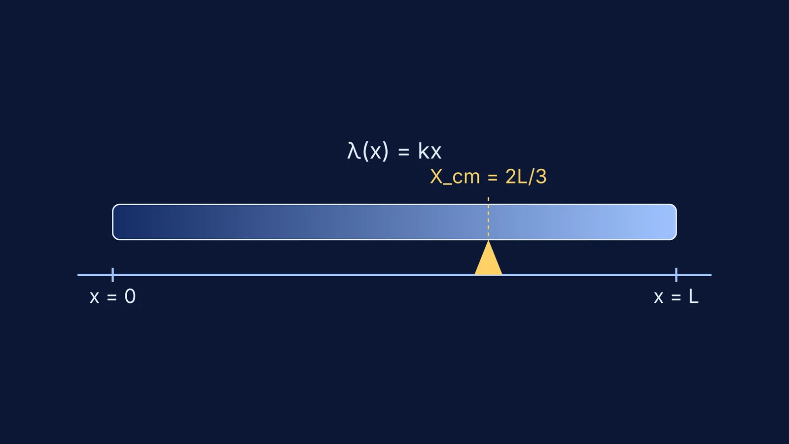
How do you find the centre of mass if λ = kx?
This is the classic case where density increases linearly from one end. The rod is extremely light at x = 0 and gets steadily heavier towards x = L. Because k is a positive constant, the density grows as you move right.
Here is the step-by-step method to solve this:
Find the total mass (M): Integrate the density function from 0 to L to find the denominator. M = ∫ kx dx = k [x² / 2] from 0 to L = kL² / 2.
Evaluate the position integral: For the numerator, multiply the density by position x and integrate. ∫ x(kx) dx = ∫ kx² dx = k [x³ / 3] from 0 to L = kL³ / 3.
Divide to find X_cm: Now, plug the numerator and denominator back into the main formula. X_cm = (kL³ / 3) / (kL² / 2) = (2/3) L.
The centre of mass is at 2L / 3. This result makes intuitive sense: because more of the rod's mass is concentrated towards the far end, the balance point shifts past the midpoint of L / 2 and rests closer to the heavier side.
How do you solve for a density λ = a + bx?
Sometimes, a rod has a baseline uniform density that gradually increases. When the density has a constant starting value a and increases by a factor of bx, the integration involves two terms but follows the exact same logic.
Find the total mass (M): Integrate the density function to find the denominator. M = ∫ (a + bx) dx = [ax + bx² / 2] from 0 to L = aL + bL² / 2.
Evaluate the position integral: Multiply the entire density function by x first. ∫ x(a + bx) dx = ∫ (ax + bx²) dx = [ax² / 2 + bx³ / 3] from 0 to L = aL² / 2 + bL³ / 3.
Divide to find X_cm: Divide the numerator by the denominator. X_cm = (aL² / 2 + bL³ / 3) / (aL + bL² / 2). To simplify this fraction, multiply the top and bottom by 6 (the common denominator of 2 and 3): X_cm = (3aL² + 2bL³) / (6aL + 3bL²). Factor out an L from the numerator: X_cm = L(3a + 2bL) / (6a + 3bL).
You can check this expression by testing a limit case. If b = 0, the rod is completely uniform with a constant density a. Plugging b = 0 into our final formula gives L(3a) / (6a), which simplifies to L / 2. This is exactly the centre of a uniform rod. Working through edge cases to test derived formulas is a habit that the Fermi Problem Library reinforces to help you catch algebraic mistakes.
Next steps
Mastering variable density integrals is about steady practice. Always start by writing down the density function, carefully setting up your bounds of integration, and remembering to divide the position integral by the total mass.
If you are brushing up on calculus techniques for physics, review how to handle u-substitution with bounds. To see another practical application of integration with varying forces, read about calculating a rod stretching under its own weight.


