

On this page
What is the angle between two lines formula?
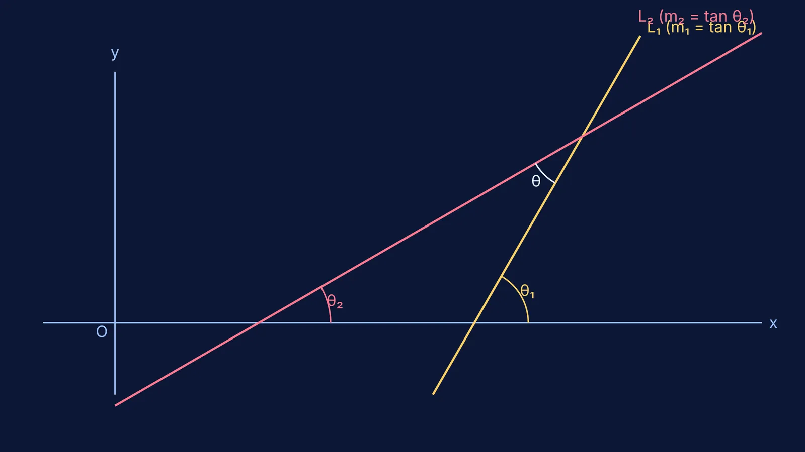
When two straight lines cross on a Cartesian plane, they form four angles around their point of intersection. Because vertically opposite angles are always equal, there are really only two distinct angles to consider: one acute angle (less than 90°) and one obtuse angle (greater than 90°). Together, these two adjacent angles lie on a straight line and therefore add up to exactly 180°.
If you know the slopes of the two lines, m₁ and m₂, the angle between them does not depend on where they intersect on the coordinate plane. According to the NCERT Class 11 Mathematics syllabus, the acute angle θ between two intersecting lines is given by the formula:
tan θ = |(m₁ − m₂) / (1 + m₁m₂)|
The absolute value (or modulus) operation ensures that the value of tan θ is always positive, which strictly corresponds to the acute angle. Once you have found this acute angle, finding the obtuse angle φ is straightforward. You simply subtract the acute angle from 180°, giving you the relationship φ = 180° − θ.
If you need a refresher on how to calculate slopes and inclinations before tackling these coordinate geometry problems, you can search for them in the Fermi Concept Library, which covers every core mathematics topic step by step.
How to use the tan theta formula
Let's walk through a practical example to see how this works. Suppose you have two lines with known slopes m₁ = 2 and m₂ = −1/3.
Plug the slope values into the angle formula:
tan θ = |(2 − (−1/3)) / (1 + (2)(−1/3))|
Simplify the terms in the numerator and the denominator:
Numerator = 2 + 1/3 = 7/3 Denominator = 1 − 2/3 = 1/3
Divide the numerator by the denominator:
tan θ = |(7/3) / (1/3)| = |7| = 7
The acute angle is therefore θ = tan⁻¹(7). The obtuse angle is 180° − tan⁻¹(7).
If you find yourself guessing whether to use the plus or minus sign during calculations, Fermi's AI tutor checks your understanding as it goes, noticing where you are stuck to help you spot algebraic slips before they derail the final answer.
What if the lines are given as ax + by + c = 0?
In exams like JEE and CBSE, straight lines are rarely handed to you as ready-made slopes. Instead, you will almost always see general equations presented in the standard form ax + by + c = 0.
For any general line equation ax + by + c = 0, the slope is determined by m = −a/b.
If you have two distinct lines, represented by a₁x + b₁y + c₁ = 0 and a₂x + b₂y + c₂ = 0, you can substitute their slopes m₁ = −a₁/b₁ and m₂ = −a₂/b₂ directly into the standard angle formula. The algebraic fractions cancel out to leave a simplified expression:
tan θ = |(a₁b₂ − a₂b₁) / (a₁a₂ + b₁b₂)|
You can use this direct formula to save time during a timed exam, or you can simply find m₁ and m₂ first and use the original slope formula. The final numerical result will be completely identical either way. For more practice on working with line equations, see our related guide on the condition for three lines to be concurrent.
Parallel and perpendicular cases
The angle formula also neatly proves the two most common and important rules of coordinate geometry.
Parallel lines: If two lines are parallel, they never intersect, meaning the angle between them is exactly 0°. Since the tangent of 0° is 0, the numerator of our angle formula must be equal to zero. This implies that m₁ − m₂ = 0, which gives the familiar rule m₁ = m₂.
Perpendicular lines: If the two lines cross at a right angle (90°), the value of tan(90°) is mathematically undefined. In any fraction, an undefined result means that the denominator must be equal to zero. Therefore, we set 1 + m₁m₂ = 0, which directly gives the perpendicularity condition m₁m₂ = −1.
When proving that three points lie on the exact same straight line, you might also use slopes to establish their collinearity, though position vectors offer another powerful way to solve this as shown in the collinear points with vectors test.
If you are struggling to picture how these different equations translate to intersecting lines on the Cartesian plane, you can graph them interactively in the Fermi Simulation Lab to see how changing a single slope instantly alters the overall angle.


