

On this page
A 2021 study of 159 physics students found that only 30.47% could correctly answer conceptual questions about acceleration when the format changed. Acceleration problems often feel like a puzzle where you have to pick the right equation from a list. But when a question gives you the distance an object covers in two back-to-back time intervals, there is a direct geometric way to the answer.
How do you find acceleration from successive equal intervals?
Suppose a car is accelerating uniformly along a straight road. It covers a distance s₁ in a time interval T, and then covers a distance s₂ in the very next time interval T.
If you use the standard equation of motion for the first interval, the distance is s₁ = uT + ½aT², where u is the velocity at the start of that interval.
By the end of the first interval, the car has sped up. Its new velocity is u + aT. The distance it covers in the second interval is this new starting velocity multiplied by the time T, plus the ½aT² term that accounts for the acceleration during that specific interval:
s₂ = (u + aT)T + ½aT² = uT + aT² + ½aT²
If you subtract the first distance from the second, the uT and the ½aT² terms cancel out completely:
s₂ − s₁ = aT²
This means the difference in distance between any two successive equal time intervals depends only on the acceleration and the time squared. The SI unit of acceleration is metre per second squared (m/s²).
Why is the difference formula useful?
In exams, questions frequently give you two distances covered in adjacent time blocks, like a stone falling past a window or a train pulling away from a station. The standard approach is to set up two simultaneous equations with two unknowns (u and a), which takes time and invites algebra mistakes.
Because s₂ − s₁ = aT² completely removes the initial velocity u from the picture, it gives you a much faster route. Once you know the acceleration, finding the initial velocity or the final velocity becomes a straightforward substitution.
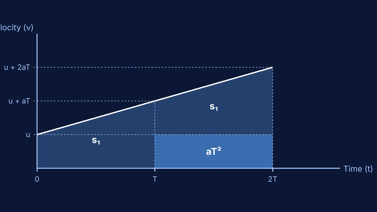
You can also see this directly on a velocity-time graph. The area under the graph for the first interval is a trapezium. For the second interval, the graph starts higher up, so the new trapezium is taller. The extra area in the second trapezium is exactly a rectangle of height aT (the increase in velocity) and width T. The area of that rectangle is aT × T = aT², proving geometrically why the distances differ by that exact amount.
What is the worked example for successive intervals?
Here is a worked example to show how the shortcut behaves in practice. A ball rolling down a ramp covers 12 m in 2 seconds, and then covers 20 m in the next 2 seconds. What is its acceleration?
Identify the time intervals. Check that they are equal, with T = 2 s in this case.
Note the distances covered: s₁ = 12 m and s₂ = 20 m.
Find the difference in distance: s₂ − s₁ = 20 − 12 = 8 m.
Set this difference equal to aT²: 8 = a × 2².
Solve for the acceleration a: 8 = 4a, which means a = 2 m/s².
If you need the initial velocity, you can substitute a = 2 m/s² back into the original distance formula for the first interval: s₁ = uT + ½aT². That gives 12 = u(2) + ½(2)(4), which simplifies to 12 = 2u + 4, leaving u = 4 m/s.
How can AI help with kinematics?
When you are faced with a blank page and a list of equations, knowing which one to apply can feel like guesswork. A step-by-step solver like the Fermi Problem Library explains the reasoning rather than printing an answer. If you are struggling to see where these ideas fit together, the Fermi Concept Library gives every concept its own lesson and its place in the map, so you can build a solid foundation.


